Overview of a steady-periodic model of modal instability in fiber amplifiers
Arlee V. Smith and Jesse J. Smith
AS-Photonics, LLC, 6916 Montgomery Ave. NE, Suite B8, Albuquerque, NM 87109
- T. Eidam, C. Wirth, C. Jauregui, F. Stutzki, F. Jansen, H.-J. Otto, O. Schmidt, T. Schreiber, J. Limpert, and A. Tünnermann, “Experimental observations of the threshold-like onset of mode instabilities in high power fiber amplifiers,” Optics Express, vol. 19, pp 23218-13224 (2011), https://www.opticsinfobase.org/oe/abstract.cfm?URI=oe-19-14-13218.
- M. Karow, H. Tünnermann, J. Neumann, D. Kracht, and P. Wessels, “Beam quality degradation of a single-frequency Yb-doped photonic crystal fiber amplifier with low mode instability threshold,” Optics Letters, vol. 37, pp 4242–4244 (2012), https://www.opticsinfobase.org/oe/abstract.cfm?URI=ol-37-20-4242.
- H.-J. Otto, F. Stutzki, F. Jansen, T. Eidam, C. Jauregui, J. Limpert, and A. Tünnermann, “Temporal dynamics of mode instabilities in high-power fiber lasers and amplifiers,” Optics Express, vol. 20, 15710–15722 (2012), https://www.opticsinfobase.org/oe/abstract.cfm?URI=oe-20-14-15710.
- B. Ward, C. Robin, and I. Dajani, “Origin of thermal modal instabilities in large mode area fiber amplifiers,” Optics Express, vol. 20, pp 11407–11422 (2012), https://www.opticsinfobase.org/oe/abstract.cfm?URI=oe-20-10-11407.
- F. Stutzki, H.-J. Otto, F. Jansen, C. Gaida, C. Jauregui, J. Limpert, and A. Tünnermann, “High-speed modal decomposition of mode instabilities in high-power fiber lasers,” Optics Letters, vol. 36, pp 4572-4574 (2011), https://www.opticsinfobase.org/ol/abstract.cfm?URI=ol-36-23-4572.
- A. V. Smith and J. J. Smith, “Mode instability in high power fiber amplifiers,” Opt. Express 19, 10180–10192 (2011), https://www.opticsinfobase.org/oe/abstract.cfm?URI=oe-19-11-10180.
- K. R. Hansen, T. T. Alkeskjold, J. Broeng, and J. Laegsgaard, “Thermally induced mode coupling in rare-earth doped fiber amplifiers,” Opt. Lett. 37, 2382–2384 (2012), https://www.opticsinfobase.org/oe/abstract.cfm?URI=ol-37-12-2382.
- K. R. Hansen, T. T. Alkeskjold, J. Broeng, and J. Laegsgaard, “Theoretical analysis of mode instability in high-power fiber amplifiers,” Opt. Express 21, 1944–1971 (2013), https://www.opticsexpress.org/abstract.cfm?URI=oe-21-2-1944.
- L. Dong, “Stimulated thermal rayleigh scattering in optical fibers,” Opt. Express 21, 2642–2656 (2013), https://www.opticsexpress.org/abstract.cfm?URI=oe-21-3-2642.
- B.G. Ward, “Modeling of transient modal instability in fiber amplifiers,” Optics Express, vol. 21, pp 12053-12067 (2013), https://www.opticsexpress.org/abstract.cfm?URI=oe-21-10-12053.
- S. Naderi, I. Dajani, T. Madden, and C. Robin, “Investigations of modal instabilities in fiber amplifiers through detailed numerical simulations,” Optics Express, vol. 21, pp 16111-16129 (2013), https://www.opticsinfobase.org/oe/abstract.cfm?uri=oe-21-13-16111.
- A. V. Smith and J. J. Smith, “Steady-periodic method for modeling mode instability in fiber amplifiers,” Opt. Express 21, 2606-2623 (2013) https://www.opticsinfobase.org/oe/abstract.cfm?URI=oe-21-3-2606.
- K. D. Cole, “Steady-periodic Green’s functions and thermal-measurement applications in rectangular coordinates,” J. of Heat Trans. 128, 706-716 (2006); DOI: 10.1115/1.2194040.
- K. D. Cole and P. E. Crittenden, “Steady-periodic Heating of a cylinder,” J. of Heat Trans. 131, 091301-1–091301-7 (2009); DOI: 10.1115/1.3139107.
- M. D. Feit and J. A. Fleck, “Computation of mode properties in optical fiber waveguides by a propagating beam method,” Applied Optics 19, 1154-1164 (1980), https://ao.osa.org/abstract.cfm?URI=ao-19-7-1154.
- M. D. Feit and J. A. Fleck, “Computation of mode eigenfunctions in graded-index optical fibers by the propagating beam method,” Applied Optics 19, 2240-2246 (1980), https://ao.osa.org/abstract.cfm?URI=ao-19-13-2240.
- Robert W. Boyd. Nonlinear Optics. Academic Press, Inc., 1992.
- A. V. Smith and J. J. Smith, “Influence of pump and seed modulation on the mode instability thresholds of fiber amplifiers,” Opt. Express 20, 24545–24558 (2012), https://www.opticsinfobase.org/oe/abstract.cfm?URI=oe-20-22-24545.
- A. V. Smith and J. J. Smith, “Maximizing the mode instability threshold of a fiber amplifier,” arXiv:1301.3489 [physics.optics] (2013), https://arxiv.org/abs/1301.3489.
- A. V. Smith and J. J. Smith, “Increasing mode instability thresholds of fiber amplifiers by gain saturation,” Opt. Express 21, 15168-15182 (2013), https://www.opticsinfobase.org/oe/abstract.cfm?URI=oe-21-13-15168.
- A. V. Smith and J. J. Smith, “Spontaneous Rayleigh Seed for Stimulated Rayleigh Scattering in High Power Fiber Amplifiers,” IEEE Photonics Journal, vol. 5, pp 7100807 (2013); DOI: 10.1109/JPHOT.2013.2280526.
- Peter W. Milonni. The quantum vacuum: an introduction to quantum electrodynamics. Academic Press, Inc., 1994.
- A. V. Smith and J. J. Smith, “Modeled fiber amplifier performance near the mode instability threshold,” arXiv:1301.4278 [physics.optics] (2013), https://arxiv.org/abs/1301.4278.
- A. V. Smith and J. J. Smith, “Mode competition in high power fiber amplifiers,” Opt. Express 19, 11318-11329 (2011), https://www.opticsexpress.org/abstract.cfm?URI=oe-19-12-11318.
- A. V. Smith and J. J. Smith, “Frequency dependence of mode coupling gain in Yb doped fiber amplifiers due to stimulated thermal Rayleigh scattering,” arXiv:1301.4277 [physics.optics] (2013), https://arxiv.org/abs/1301.4277.
- A. V. Smith and J. J. Smith, “Mode instability thresholds of fiber amplifiers,” Photonics West Conf. Fiber Lasers X, paper 8601-108 (2013).
1. Introduction
Mode instability refers to the degradation of the output beam profile from large mode area fiber amplifiers for powers above a sharp threshold. The instability has been observed by several researchers [1,2,3,4,5] in Yb$^{3+}$-doped silica fiber amplifiers pumped at $976\, \rm{nm}$ and operating in the signal wavelength range $1030-1080\, \rm{nm}$. Reported instability thresholds lie in the range of $100$ W to $2500$ W.
We have developed a physical model that we believe explains this behavior, and we have constructed a numerical model capable of precise predictions of the amplifier behavior, including instability thresholds.
2. Physical mechanism (STRS)
We attribute the degradation in beam quality to the exponential growth of higher order modes via stimulated thermal Rayleigh scattering (STRS) [6]. The physical basis of STRS is that two populated transverse modes interfere to produce an irradiance grating along the fiber with a period equal to the beat length between the two modes. The presence of the irradiance grating means different regions within the doped fiber core have different transverse profiles of signal irradiance and thus different population inversions and thus different pump absorption and thus different heating rates supplied by the quantum defect fraction of the absorbed pump light. This mechanism implies that higher signal irradiance is associated with greater heating.
The heat grating in turn leads to the formation of a temperature grating which, via the thermo-optic effect, creates a weak refractive index grating that can couple light between the two interfering modes. Usually the fundamental mode ($\rm{LP}_{01}$) contains the highest power and it couples most strongly with mode $\rm{LP}_{11}$, so $\rm{LP}_{11}$ is the mode that usually appears suddenly at the instability threshold.
A crucial aspect of STRS is that power transfer between the modes requires a phase shift between the irradiance grating and the thermally induced refractive index grating. This shift can occur if the frequencies of the interfering modes differ and their propagation constants also differ. The velocity of the irradiance grating is then \begin{equation} {v}=\frac{2\pi \Delta \nu}{\Delta \beta} \end{equation} where $\Delta \nu$ is the frequency difference of light in the two modes and $\Delta \beta$ is the difference in the two modal propagation constants. The moving temperature grating lags the moving irradiance grating because it takes time to develop via heat accumulation and thermal diffusion. This time lag provides the phase shift necessary for power transfer between modes. A quick estimate of the time lag is that it is roughly equal to the thermal diffusion time across the fiber core, given by \begin{equation} \tau=\frac{r^2C\rho}{\kappa} \end{equation} where $r$ is the radius, $C$ is the specific heat, $\rho$ is the mass density, and $\kappa$ is the thermal conductivity of the core. Using the thermal characteristics of silica this becomes \begin{equation} \tau=1.12r^2 \end{equation} where $\tau$ is in microseconds and $r$ is in micrometers. For large mode area fibers $\tau$ is $100-5000$ $\mu$s, so a large phase shift between irradiance and temperature requires a frequency offset of roughly $1/\tau$, or $200-10000$ Hz.
For large core, step index fibers with a low numerical aperture (NA=$0.05$ is typical) the grating velocity is quite slow compared with most velocities encountered in optics. A runner or bicyclist could keep pace. The direction of grating travel depends on the relative signs of $\Delta \nu$ and $\Delta \beta$. For modes $\rm{LP}_{01}$ and $\rm{LP}_{11}$ the motion is downstream if the $\rm{LP}_{11}$ light is red shifted relative to the $\rm{LP}_{01}$ light. Downstream grating motion causes a phase shift that leads to power transfer from $\rm{LP}_{01}$ to $\rm{LP}_{11}$. If $\rm{LP}_{11}$ is blue shifted, the motion is upstream, and the direction of power transfer is reversed. The light transferred between modes is also frequency shifted by the moving grating, so it assumes the frequency of its new home. These mode coupling rules were outlined in ref. [6]. Other authors have published alternate formulations of the same underlying physics [7,8,9,10,11].
3. Steady-periodic modeling method
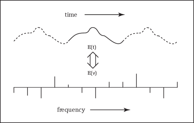
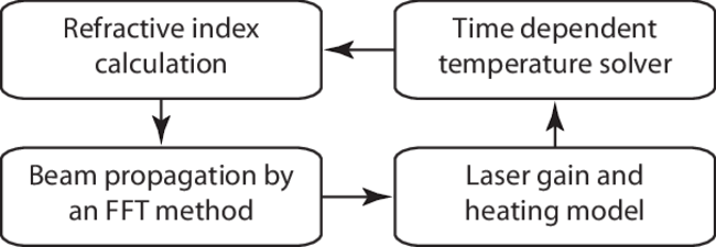
Based on the physics of mode coupling just outlined, the required elements of a mathematical model of the STRS process are (1) a laser gain and heating model, (2) a time-dependent temperature solver, and (3) a beam propagator that takes account of the temperature-induced refractive index changes. We are primarily interested in studying the performance of CW or quasi-CW amplifiers rather than transient behaviors caused by sudden changes in seed or pump power, because our target application is coherent and spectral beam combining on time scales of $100$ ms and longer. However, time dependence is still required in the model because the frequency shifts necessary for STRS gain must be included. We use a steady-periodic assumption to account for the frequency shifts. This assumption means the time dependence of the modal beat at each $z$ location is taken to be perfectly periodic. The modeled period must be made long enough to include the smallest frequency offset of interest, and it must be divided into fine enough time slices to resolve the largest frequency span of interest. Because a fixed time period is used, the signal spectrum comprises a set of uniformly spaced frequencies separated by the inverse of the period. However, because any time period can be chosen, any frequency spacing can be selected. Of course, more frequencies usually means longer run times, so we try to judiciously limit the frequencies to the minimum number required to capture the physics of interest. Figure 1 illustrates the time/frequency consequences of the steady-periodic assumption.
The temperature profile $T(x,y,t)$ at each $z$ location is solved over one temporal cycle, and the resulting temperature-induced, time-periodic index grating is used to propagate each of the corresponding time slices of the optical field over a single $\Delta z$-step. This is repeated for each $z$ to integrate along the length of the fiber. At the end of a model run we have a record along the full length of the fiber and over one full time period of all the modal amplitudes, plus the pump power. We also save temperature and electric field values for a few transverse positions. From this information we can produce movies of the optical field and temperature evolution along the fiber. These movies are featured in the descriptions below.
The integration process just outlined is diagrammed in Figure 2. We will describe each of the four components briefly in the next sections. Reference [12] gives full details of our model. Our philosophy is to keep each part of the model as general as possible, minimizing the number of assumptions about the fiber, the pump or seed light, the cooling and bending of the fiber, etc. This approach makes it relatively easy to add various physical effects without extensive modification of the model.
4. Laser gain & heating calculation
We compute the population inversion $[n_u(x,y,t)-n_l(x,y,t)]$ at each $z$ location making the assumption that the population has assumed its steady state level at each time point. This is a good assumption because the effective upper state lifetime in a high power amplifier is usually much shorter than the characteristic time period for STRS. The computed population inversions are then used to compute the absorbed pump power over one $\Delta z$-step for each time slice, assuming the pump power is uniformly distributed throughout the pump cladding. The heat is computed from the difference in pump plus signal power entering and leaving the $\Delta z$-step within the time slice of interest. A linear absorption profile $\alpha(x,y,z)$ can also be included, for instance to consider heat deposited due to photodarkening. Scattering losses of the signal, if any, are assumed to contribute no heat.
5. Temperature & refractive index calculation
The assumption of steady-periodic heating allows us to use a steady-periodic Green's function method to compute the time-dependent temperature profiles at each $z$ location [13,14]. This is a fast method of solving the temperature equation, and was the motivation for making the steady-periodic assumption. A
6. Beam propagation calculation
We use a fast Fourier transform beam propagation method [15,16] (FFT BPM) to propagate each time slice of the optical field within a single period, as described in ref. [12]. The spatial grid is usually square and we use a rectangular mesh. Numerical beam propagation has the advantage of including all fiber modes, both bound and radiative, because the light in all modes with all frequencies is included in a single time-dependent field that is propagated in the presence of the time-dependent refractive index profile without the necessity of decomposing the field into modes and frequencies.
The use of such a general propagation method means the model can easily handle such physical effects as mode distortion due to fiber bending, asymmetric cooling, bend losses, photodarkening, linear loss, scattering loss, thermal lensing, $n_2$ effects, and any set of transverse modes. Its drawback is that the $\Delta z$-step must be much smaller than the modal beat length. Typical step sizes are a few microns. Fortunately, FFTs can be extremely fast so this is a practical approach. It is an oft repeated myth that beam propagation methods are too computationally intensive to incorporate into a useful model, and that as a consequence faster alternatives are necessary. Our model runs in as little as 15 minutes for a 1.2 m long amplifier on a $600 desktop computer (with Intel Core i7-3770 CPU) using the freely available Gnu Fortran compiler, OpenMP, and FFTW [12]. Parallel computation is facilitated in this model. The BPM, heating, and refractive index calculations are all parallel in $t$ while the temperature calculation is parallel in $(x,y)$.
7. Frequency dependence of STRS gain
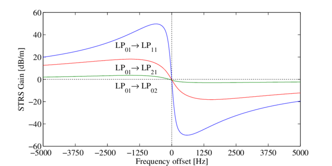
The model just outlined predicts an STRS gain profile for any mode pair. The gains have frequency dependences that are typical of stimulated thermal Rayleigh scattering processes [17]. An example is shown in Figure 3. As seen in the plot, the gain for coupling from the fundamental mode to a higher order mode is positive for red detuning of the higher order mode and negative for blue detuning. For light in $\rm{LP}_{01}$ the coupling is usually strongest to mode $\rm{LP}_{11}$. The STRS gain is zero for zero frequency shift, but laser gain (not included in this figure) is present and is nearly uniform across the frequency range of interest for STRS. Laser gain is typically on the order of a few decibels per meter, while STRS gain can be many tens of decibels per meter, depending on the fiber parameters and operating conditions.
The general shape of the gain curve is easily understood. For small frequency shifts the phase shift between the temperature and irradiance gratings is nearly linear in grating velocity or frequency offset. This leads to nearly linear increase in gain. As the frequency shift increases beyond the point of maximum gain, the time of passage of one period of the irradiance grating becomes short relative to the temperature response time so the temperature grating weakens and gain diminishes.
8. Sources of frequency shifted seed light
The STRS process produces exponential gain of red-shifted higher order modes, but those modes must be seeded at a nonzero power level in order to be amplified to the mode instability threshold. Here we discuss four sources that can seed the process.
8.1 Amplitude modulation of injected signal
When the signal is injected into the amplifier, some fraction of it will almost always be accidentally injected into the higher order modes. If the signal has no amplitude modulations, this population of both the $\rm{LP}_{01}$ and $\rm{LP}_{11}$ modes creates a static irradiance grating that does not lead to STRS gain. However, if the signal is amplitude modulated, the irradiance grating oscillates in time. The oscillating part of the standing wave grating can be decomposed into equal amplitude waves moving upstream and downstream. If the frequency of modulation is in the STRS gain band, the grating moving upstream will be deamplified and the grating moving downstream will be amplified. Thus, amplitude modulation of the signal can serve as the required seed [8,18,19,20].
One important point is that phase modulation of the input signal, rather than amplitude modulation, does not initiate STRS. This was first demonstrated by Hansen [8] and we expand upon this point later in this article. Phase modulation does not cause oscillation of the irradiance grating created by accidental seeding of a higher order mode because the difference in phase between the two modes is constant in time. Therefore, there is no moving grating to provide STRS gain.
8.2 Amplitude or spectral modulation of pump light
Amplitude modulation of the seed light can also be induced by an amplitude or spectrally modulated pump. An amplitude modulated pump produces modulation of the signal in all populated transverse modes via modulated laser amplification. The resulting red AM sidebands in the higher order mode can be amplified by STRS just as described above. Similarly, if the pump spectrum is modulated, because of the narrowness of the pump spectral absorption peak, this may translate into amplitude modulation of the pumping rate and thus of the signal power.
8.3 Spontaneous thermal Rayleigh scattering
The spontaneous thermal Rayleigh scattering (sTRS) process scatters light between modes while also adding frequency shifts. It is caused by thermodynamic fluctuations in temperature across the core of a fiber, and it produces amplitude modulated scattering between the modes. Like quantum noise this produces low power noise that is spectrally broad compared with the STRS gain bandwidth. For any pair of modes the power spectrum of the sTRS coupling rate can be computed, and the rate near the peak frequency of the STRS gain curve can be found [21]. sTRS scattering is distributed along the fiber. The power scattered into the higher order mode from $\rm{LP}_{01}$ is proportional to the $\rm{LP}_{01}$ power. The scattering rate is also proportional to $T^2$, and is nearly constant as a rate per beat length for all step index, large mode area fibers. At room temperature this seed is perhaps $100-1000$ times greater than the quantum noise level, so sTRS seeding is expected to dominate unless signal or pump amplitude modulation is present.
8.4 Quantum noise seed
Quantum noise, or shot noise, is well understood, and a stochastic quantum electrodynamic method [22] is straightforward to apply. Quantum noise fills each spatial mode with one half photon per time step. This means it also provides one half photon of energy to each comb frequency in our model, giving each an average power of $h\nu\delta\nu/2$ where $\delta \nu$ is the comb spacing. The approximate total effective quantum noise seed is thus $h\nu\Delta\nu/2$ where $\Delta \nu$ is the effective width of the STRS gain peak. In our model we populate all the comb frequencies of each mode with random Gaussian light of average power $h\nu\delta \nu/2$ as an initial condition. The injected fields are added to these noise fields. Quantum noise produces amplitude modulation at a low level in each mode, and this serves to seed the STRS process.
Although quantum noise is not expected to be the dominant seed source in actual amplifiers, it is often used as the seed in numerical models because it is easy to implement and because it facilitates comparisons among models. In many of the discussions below we use quantum noise seeding with the knowledge that it is unlikely to be exact, but it forms a constant starting seed to allow quantitative comparisons of the influence of other physical effects such as photodarkening, population saturation, etc.
9. Example threshold calculations
| $d_{\rm core}$ | $74\, \mu \rm{m}$ | $d_{\rm dope}$ | $74\, \mu \rm{m}$ |
| $d_{\rm clad}$ | $170\, \mu \rm{m}$ | $N_{Yb}$ | $3.5\times 10^{25}\, \rm{m}^{-3}$ |
| $\lambda_p$ | $977\, \rm{nm}$ | $\lambda_s$ | $1064\, \rm{nm}$ |
| $\sigma_p^a$ | $1.53 \times 10^{-24}\, \rm{m}^2$ | $\sigma_p^e$ | $1.87 \times 10^{-24}\, \rm{m}^2$ |
| $\sigma_s^a$ | $6.00 \times 10^{-27}\, \rm{m}^2$ | $\sigma_s^e$ | $3.58 \times 10^{-25}\, \rm{m}^2$ |
| ${P}_p$ | $\rm{varies}$ | $\rm{Total}\, {P}_s$ | $14.7\, \rm{W}$ |
| $dn/dT$ | $1.2 \times 10^{-5}\, \rm{K}^{-1}$ | $L$ | $1.15\, \rm{m}$ |
| $\rho$ | $2201\, \rm{kg/m}^3$ | $C$ | $702\, \rm{J/kg}\cdot \rm{K}$ |
| $n_{\rm core}$ | $1.45031$ | $n_{\rm clad}$ | $1.45$ |
| $\tau$ | $850\, \mu \rm{s}$ | $K$ | $1.38\, \rm{W/m}\cdot\rm{K}$ |
| $NA$ | $0.03$ | $V$ | $6.55$ |
| $A_{\rm eff}$ | $2748\, \mu\rm{m}^2$ |
9.1 Baseline case
We usually apply our STRS model only to the determination of mode instability thresholds because these thresholds are of primary import to most fiber amplifier users. Our model can be readily applied to conditions slightly above threshold [23], and it should be applicable, with more effort, to operation well above threshold, although we do not have extensive experience in doing so.
This paper is intended to illustrate the general physical principles of STRS and the general capabilities of our model, so we are not concerned with the exact power levels or other details of the amplifier and operating conditions. However, all plots and movies will be for amplifiers similar to the baseline case used to generate Figs. 4 and 5 with the parameters given in Table 1. In subsequent sections, input seeding conditions will be altered and the pump power will be adjusted as necessary to achieve threshold. We define the threshold as 1% of the signal in the frequency-shifted higher order mode.
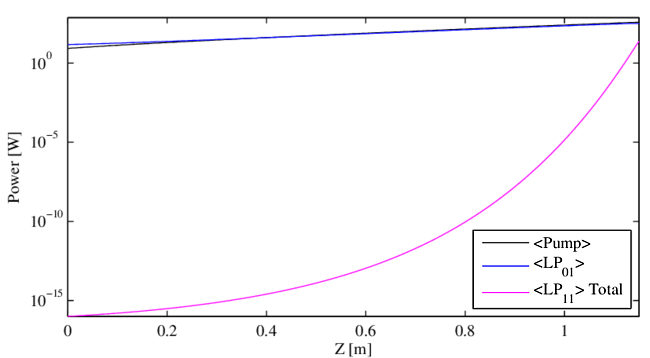
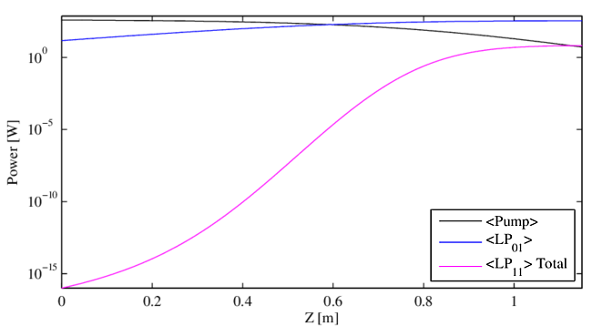
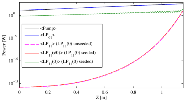
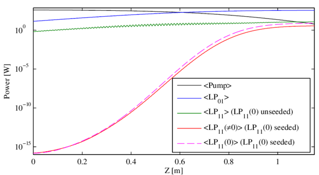
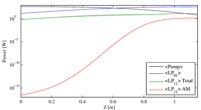
Figure 4 shows the power, averaged over one period, in the pump and in modes $\rm{LP}_{01}$ and $\rm{LP}_{11}$ along the length of the counter-pumped amplifier. Figure 5 shows the same for the co-pumped amplifier. Here, the injected light is monochromatic in both seeded modes, but there is a frequency shift between the two seeds. We use the notation LP$_{11}(\nu)$ to indicate the power injected into $\rm{LP}_{11}$ at a frequency shift of $\nu$ relative to the main signal injected into LP$_{01}(0)$. In Figures 4 and 5, we seed with $14.7$ W in LP$_{01}(0)$, and $10^{-16}$ W in LP$_{11}(\nu_m)$ to approximate the quantum noise level, where $\nu_m = -550$ Hz is the frequency of maximum STRS gain. For the counter-pumped case, the input pump power at threshold is $365$ W. For the co-pumped case, the input pump power at threshold is $386$ W. In the counter-pumped case, the signal experiences $13.5$ dB of laser gain, growing to $332$ W at output. In the co-pumped case, the signal grows to $354$ W at output, a laser gain of $13.8$ dB. STRS gain in each case is much larger: for the counter-pumped amplifier $\rm{LP}_{11}$ output power is $3.51$ W for a gain of $165.4$ dB, while for co-pumped $\rm{LP}_{11}$ output power is $3.81$ W for a gain of $165.8$ dB.
9.2 Quantum noise seeding
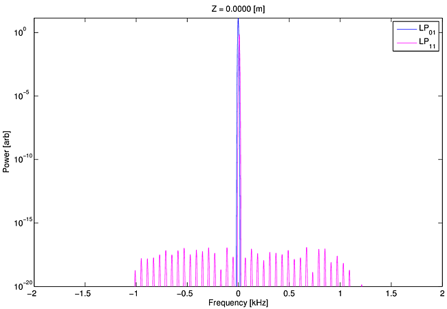
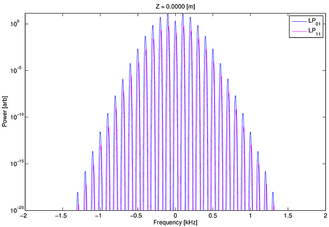
In Movie 1 we show the evolution of the signal spectrum for perfect launch of a monochromatic seed into $\rm{LP}_{01}$. Only $\rm{LP}_{01}(0)$ contains injected signal light. Quantum noise alone seeds a broad range of frequencies of $\rm{LP}_{11}$. In this model run we make no assumptions about frequency shifts or gain spectra. The movie shows the evolution of the spectra of modes $\rm{LP}_{01}$ and $\rm{LP}_{11}$ as the light propagates along the fiber. The pump power is chosen to lie near the instability threshold. The spectral powers are displayed on a log scale in order to display the extremely wide power range extending from the starting quantum noise level of around $10^{-17}$ W per frequency bin to the threshold level of order $1$ W.
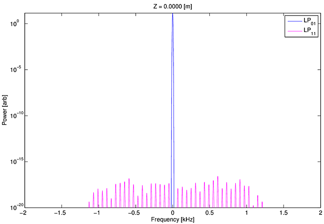
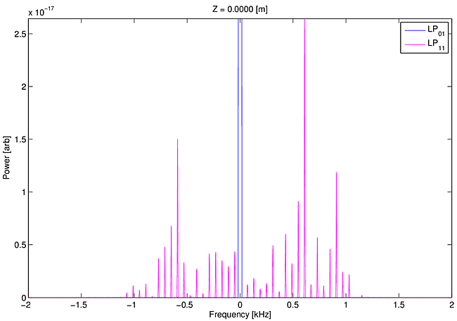
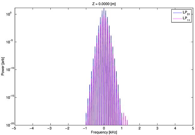
Movie 1 clearly shows that the Stokes shifted noise in $\rm{LP}_{11}$ is amplified, and that the maximum amplification occurs at a frequency shift of -550 Hz. Because of nonlinearities in the population equations, and thus in the heat deposition, additional frequencies are continuously generated in both $\rm{LP}_{01}$ and $\rm{LP}_{11}$. On the log scale used for this movie the spectral development looks rather complicated. However, when the same information is displayed on a linear scale in Movie 2 the amplification of a spectrally narrow and Stokes shifted $\rm{LP}_{11}$ signal is more apparent.
The important lesson from Movies 1 & 2 is that a red shift for the amplified $\rm{LP}_{11}$ light is self selected by the model without any nudges from the modelers. Beam propagation effects combined with thermal delays are by themselves entirely sufficient to guarantee this selection. There is no mechanism by which we explicitly enforce amplification of certain frequencies.
Movie 2 also demonstrates that, near threshold, only a narrow range of frequencies of $\rm{LP}_{11}$ are amplified. This suggests we might be able to compute thresholds quite well using a single frequency lying near the gain peak. The appropriate starting power is then $h\nu\Delta \nu/2$ where $\Delta \nu$ is the effective width of the gain peak, rather than a set of frequencies spaced as in Movie 2. We have verified that threshold powers computed these two ways agree within three percent. Because our model runs faster using the single frequency stand-in, many of our threshold studies use the single frequency approximation.
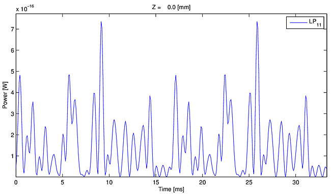
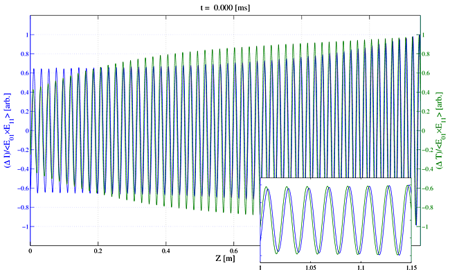
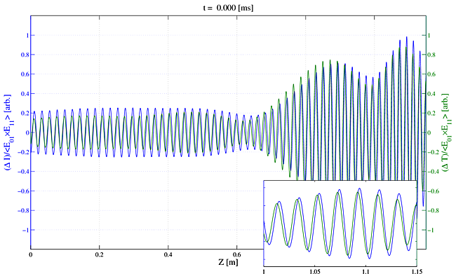
We can also follow the evolution of a single period of power in $\rm{LP}_{11}$ as it propagates along the fiber. Two cycles of the periodic behavior are displayed in Movie 3. Although our method imposes perfect periodicity on the $\rm{LP}_{11}$ field (and power) at each $z$ location, its time profile within the period evolves as it propagates along the fiber.
In Movie 4 we show how the irradiance and temperature gratings move when using a single frequency seed as a stand-in for quantum noise in $\rm{LP}_{11}$. The gratings are calculated from the differences in temperature or irradiance at two points symmetric about the center of the core. In this movie the curves have been normalized by the grating strength averaged in time $< E_{01}\times E_{11} >$. The gratings are seen to move downstream, and the crucial phase lag between the irradiance grating and the temperature grating is evident.
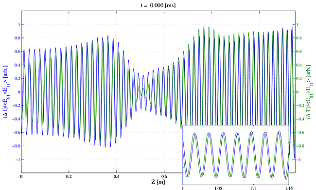
The gratings become a bit more complicated when quantum noise seeding is used rather than the stand-in single frequency seed. This is shown in Movie 5. However, close inspection of Movie 5 reveals that the essential character of a pair of moving gratings with a phase lag of temperature relative to irradiance is unchanged from Movie 4.
Just for fun we also illustrate deamplification of blue tuned $\rm{LP}_{11}$ light. In Movie 6 we seed only $\rm{LP}_{11}(+500$ Hz$)$ with $10^{-16}$ W. The movie shows that near the input end of the fiber the gratings move upstream, as expected for a deamplification of blue shifted $\rm{LP}_{11}$ light. Nonlinearities populate $\rm{LP}_{11}(-500$ Hz$)$ and after $0.5$ m the gratings both reverse direction and move downstream, as expected for amplification of the red shifted $\rm{LP}_{11}$ light. The point near $0.5$ m is simply the point where the power in the waxing red shifted $\rm{LP}_{11}(-500$ Hz$)$ light overtakes that in the waning blue shifted $\rm{LP}_{11}(+500$ Hz$)$ light. The gratings moving downstream become stronger than those moving upstream at that point.
9.3 Quantum noise plus $\rm{LP}_{11}(0)$ seeding
In practice, seeding $\rm{LP}_{11}(0)$ is almost certain to occur at some level because of the impossibility of perfect mode matching of the seed light to the fundamental mode of the fiber. The question is whether its presence affects the instability threshold. To test this we add strong $\rm{LP}_{11}(0)$ seed to the quantum noise seed.
Figures 6 and 7 and show the average power versus $z$ for $\rm{LP}_{11}(0)$ along with the sum of the $\rm{LP}_{11}$ powers at shifted frequencies, $\rm{LP}_{11}(\ne 0)$. Clearly $\rm{LP}_{11}(0)$ does not experience STRS gain. Its gain is similar to that of the fundamental mode, which is laser gain only. Close inspection reveals that its gain is actually slightly less than that of the fundamental mode due to a mode competition effect [24]. Gain of the frequency shifted light $\rm{LP}_{11}(\neq 0)$ is nearly identical to the gain found earlier with $\rm{LP}_{11}(0)$ unseeded. We conclude that the presence of the $\rm{LP}_{11}(0)$ seed has a negligible influence on the threshold.
In Movie 7 we show spectral evolution along the fiber when $\rm{LP}_{11}(0)$ is seeded with $5$% of the input signal, the remaining $95$% going into $\rm{LP}_{01}(0)$. This movie reinforces the observation $\rm{LP}_{11}(0)$ does not influence the threshold significantly due to its zero STRS gain.
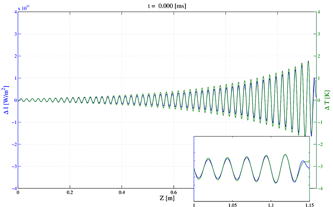
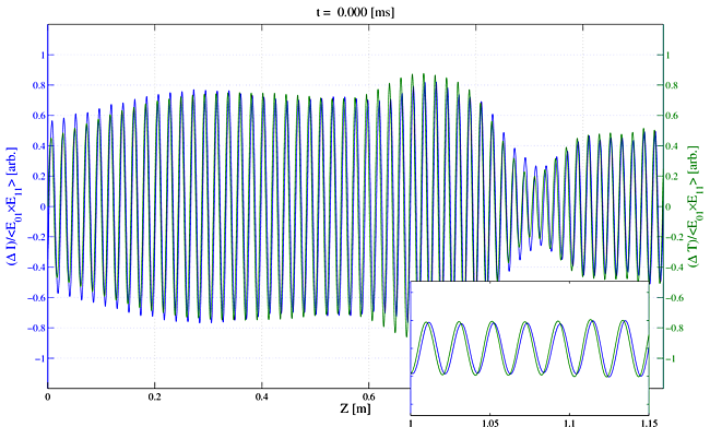
In Movie 8 we show the irradiance and temperature gratings when $\rm{LP}_{11}(0)$ is again seeded with $5$% of the input signal, and a single frequency stand-in is used in place of quantum noise. The gratings appear to be stationary for most of the fiber length, but after a certain length the gratings begin to move downstream in the usual fashion. This transition is not a magic point where mode coupling commences. When we subtract the DC portion of the grating, we obtain the result shown in Movie 9, illustrating that hidden under the strong static grating there is a moving grating with the usual properties required for STRS gain.
9.4 Phase modulated seed (no quantum noise or sTRS)
We stated earlier that a purely phase modulated input signal would not seed the STRS process. The physics argument is that the lack of amplitude modulation on the seed implies that there is no time-dependent refractive index grating and thus no STRS gain. The condition of zero amplitude modulation requires that we ignore for the moment the quantum noise background. In our model we can model this admittedly unphysical case by not including quantum noise and making the seed purely phase modulated. We have done this to generate Movie 10 which shows that a purely phase modulated seed does not seed STRS and does not lead to mode instability. Adding in the quantum noise produces a mode instability threshold equal to that for a monochromatic seed, as in Movie 11 and Figure 8. The lesson is that amplitude modulation is the critical factor for STRS initiating, not simply the presence of frequency shifted light in the gain band. This implies that a simple measurement of the signal and pump amplitude modulation in the STRS gain band (roughly $0-10$ kHz) will determine the contribution of amplitude modulation to seeding STRS.
10. Model approximations and limitations
We have already explained the steady-periodic approximation. It is important to also understand certain other approximations of our model.
10.1 Thermal boundary condition
An efficient but sufficiently accurate thermal model requires judicious choice of the thermal boundary location and boundary conditions. Because mode coupling depends only on the temperature variations within the core relative to the mean core temperature, the relevant thermal length scale is the core diameter. A thermal boundary removed from the fiber center by only a few core diameters should provide suitable accuracy. The temperature oscillations within the core region associated with STRS would not be influenced much by such a boundary.
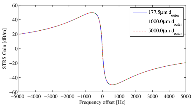
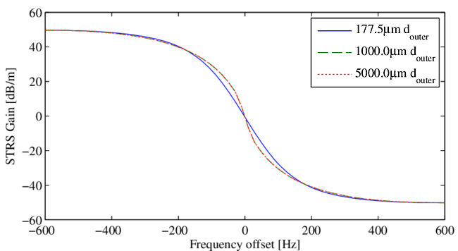
Recent updates of our model allow us to alter the location of the thermal boundary with very little performance penalty. Using this updated model to calculate the STRS gain as a function of frequency offset shows that larger thermal boundaries makes very little difference in general (see Figure 9). The only noticeable difference occurs at low frequency offsets (see Figure 10) when the outer cladding diameter is increased from $177.5\, \mu\rm{m}$ to $1000\, \mu\rm{m}$. The change is negligible near the gain maximum.
Ideally the shape of the thermal boundary should be circular to match the symmetry of the physical boundary, assuming the full boundary is cooled. However, a square boundary a few core radii away is acceptable, and that is what we use. If the fiber is cooled asymmetrically, by contact with a heat sink on one side, for example, a Green's function computed for cooling on one side of the square grid may again provide reasonable accuracy.
We have checked the steady-periodic Green's function temperature profiles by comparing them with calculations using an alternating-direction implicit method (ADI) with enforcement of the steady-periodic condition [18]. The two methods produced thresholds that differ by less than $1$%.
10.2 Counter-pumped amplifiers
A physical system with gain, time delay, and negative feedback can form an oscillator if the gain is sufficient. The oscillation frequency is determined by the time delay. Fiber amplifiers probably do not form such oscillators, but the presence of time delayed feedback, combined with amplifier gain could influence the amplifier stability. In the case of a fiber amplifier, feedback would be due to changes in the signal or pump power near the output end of the fiber leading to altered conditions earlier in the fiber. This can happen only in counter-pumped amplifiers where the pump light can carry feedback information toward the signal input end. This is difficult to model because the pump boundary condition applies to the output end of the amplifier.
For example, if the pump absorption is smaller when $\rm{LP}_{11}$ is populated near the output end, the pump power early in the fiber is increased when power switching into $\rm{LP}_{11}$ begins. This would tend to move the irradiance grating upstream, decreasing the power transfer into $\rm{LP}_{11}$, a negative feedback response. It would be strongest in fibers with confined doping where $\rm{LP}_{01}$ overlaps the dopant profile better than $\rm{LP}_{11}$. However, there is also a response with the opposite sign; higher pump power early in the fiber tends to increase the power switching if the grating motion is not altered, as would be the case near the signal input end. The net effect is unclear. It may be that feedback plays a role in the large excursions in modal power content sometimes observed in counter-pumped amplifiers operated above threshold [1,3]. However, mode instability has been documented in both co- and counter-pumped amplifiers at similar powers, and confined doping is known to raise the threshold, so feedback must play a minor role in determining instability thresholds.
10.3 Temperature dependent effects
We ignore temperature dependent effects other than the thermo-optic effect. These include the temperature dependence of the Yb$^{3+}$ absorption and emission cross sections, thermally-induced strain leading to changes in the refractive index due to the photo-elastic effect, and temperature dependence of thermal conductivity and heat capacity. Such neglected effects are expected to be insignificant compared with the thermo-optic effect.
10.4 Steady state populations
We assume the Yb$^{3+}$ ion population response to the optical fields is much faster than the thermal response. The effective lifetime of the ions is reduced from its natural value of approximately $1$ ms due to the strongly saturating fields. We use a steady state solution for the upper state population based on the instantaneous optical fields. This assumption could be removed in the steady-periodic model by integrating population rate equations, but we have not done so.
10.5 Uniform pump distribution
We make the assumption that the transverse profile of the pump is uniform across the pump cladding and thus across the core of the fiber. We believe this is an adequate approximation for cases where the pump cladding is much larger than the core. However, at very low cladding-to-core ratios this may be unrealistic.
10.6 Dispersion ignored
We do not include the group velocity difference of the modes in our model. This would become important when the signal linewidth becomes large enough that the temporal walk off between modes become comparable to the signal linewidth. Walk off is typically of order $1$ ps/m so in a few meter long amplifier a signal line widths greater than $100$ GHz may tend to alter the irradiance grating. However, only the high frequency components are affected. The slow-responding temperature grating will remain unchanged, as will the STRS gain.
10.7 sTRS seeding
We have not yet incorporated our sTRS noise model into the gain model. We still use quantum noise level seeding instead. Adding sTRS seeding should produce thresholds lower by $5-15$% and should make the threshold weakly dependent on the core temperature at the signal input end of the fiber. Accurate sTRS modeling requires knowledge of the core temperature near the signal input and this experimental information is not readily available.
10.8 Step-index approximation
The current version of the model is limited to fibers with low refractive index contrasts. It can be modified to handle photonic crystal and other fibers with high contrast by replacing the FFT based beam propagator. A vectorized, finite-difference beam propagator with conformal meshes could be used to treat high-contrast refractive index profiles.
10.9 Numerical noise
We use double-precision floating point representations of variables in our model, and this can introduce truncation errors. This numerical noise acts as a low-level broadband noise source ($10^{-30}$ W or so). We believe this level is set by the truncation error introduced in the field variables, which have the typical double-precision dynamic range of roughly $160$ dB, and the field variables are squared to obtain powers -- meaning the dynamic range of our power variables is around $320$ dB. From the typical field power variable of $10-1000$ W, a reduction by $320$ dB yields $10^{-31}$ W - $10^{-29}$ W. If all other seeds are set to zero, this very low level seed can manifest itself as modal instability behavior at sufficiently high signal powers.
11. Managing the STRS threshold
A primary purpose of our model is to provide practical guidance for raising the instability threshold. Effects that have been shown to raise the threshold include reducing the quantum defect, enhancing population saturation, confining the doping to the center of the fiber core, reducing pump and input signal amplitude modulation at frequencies in the STRS gain band, and selective mode loss via bending or fiber index design. Several of these effects are discussed below in more detail.
11.1 Pump or seed modulation
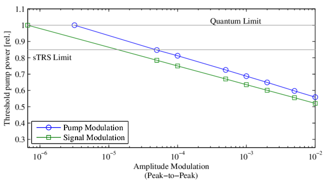
Pump or seed amplitude modulation can reduce the instability threshold substantially. In Figure 11 we plot instability threshold powers versus pump and seed modulation levels from ref. [20]. The maximum threshold would be achieved by ensuring the amplitude-modulated sideband power in $\rm{LP}_{11}$ is less than the sTRS seed. It is disappointing that no published experimental reports include measurements of what goes into the fiber in terms of pump and signal amplitude modulations. This oversight prevents precise comparisons of experimental and modeled thresholds.
11.2 Photodarkening or linear absorption
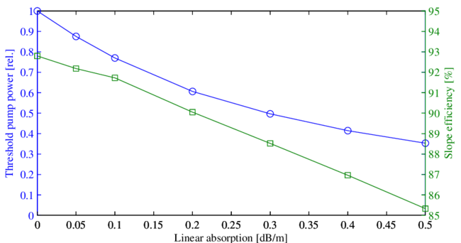
Linear absorption that converts signal light to heat can markedly reduce thresholds. Figure 12 shows the threshold reduction for linear signal absorption that is uniform across the core. It is interesting that no published experimental reports provide a precise accounting of absorbed pump power even though measured efficiencies are often in the range of $75-85$% compared with the quantum defect of $92$% or so. This oversight also hinders comparisons of experimental and model thresholds.
11.3 Population saturation
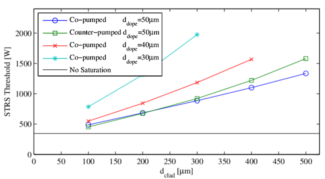
The spatial profile of the deposited heat computed from the pump absorption is proportional to $[\sigma_p^an_l(x,y)-\sigma_p^en_u(x,y)]$ which can differ strongly from the signal irradiance profile if the population inversion is depleted by transverse spatial hole burning, as was shown in [20]. Figure 13 presents an example of the modeled effects of saturation on mode instability thresholds.
It is an important point that efficient fiber amplifiers, operating above a few watts, generally have strong transverse hole burning at some or all positions along the fiber. This strong effect must be included for accurate modeling.
11.4 Mode specific loss
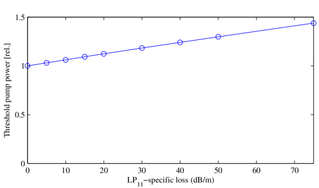
It is often noted that fibers with guiding losses for the higher order modes should have higher instability thresholds or avoid instability altogether. However, high loss is required to raise the threshold because of the enormous STRS gain at threshold. Figure 14 shows the threshold dependence on $\rm{LP}_{11}$ loss for an amplifier approximately one meter in length [26]. Mode selective loss would be more effective in longer fibers.
11.5 Future studies
Numerous other physical effects can be modeled but have not yet been thoroughly studied. They include mode distortion due to fiber bending, bend loss, asymmetric cooling boundary conditions, measured pump and seed modulation, and index profiles other than a step index. All can be modeled using same general method.
12. Observations and conclusions
We list here several important conclusions regarding mode instability drawn from hundreds of model runs including those described in the preceding sections.
The STRS Stokes shift can occur automatically. When we seed $\rm{LP}_{11}$ with only quantum noise and do not preselect in any way which frequencies experience STRS gain, the model produces gain in $\rm{LP}_{11}$ at the expected Stokes shifted frequencies.
Moving irradiance and temperature gratings are observed whenever STRS gain is present. These moving gratings are sometimes masked by static gratings, but when the static grating is subtracted the moving gratings are always present.
Stationary gratings do not affect STRS gain or mode instability thresholds. The STRS threshold is nearly independent of power in $\rm{LP}_{11}(0)$ in the absence of pump or signal modulation.
Quantum noise or sTRS seeding produces realistic thresholds. Our model predicts thresholds consistent with those reported in the literature when the seed is quantum noise or sTRS. It is not yet possible to test the model precisely against measured thresholds because the measurements do not include adequate documentation of modulation of the seed or pump, or of the overall optical power budget.
The Stokes shifted light in $\rm{LP}_{11}$ shows continuous gain along the length of the fiber, without any discontinuities.
Only the AM portion of the seed within the gain band is amplified. Any amplitude modulation in the gain band of STRS seeds the STRS process. A phase modulated seed was shown to be incapable of initiating STRS.
Photodarkening can lower the threshold. We have shown that a photodarkening absorption of less than a few dB can lower the threshold by a factor of $3$, with only a small corresponding loss in output power. We demonstrated this using an unrealistic photodarkening model. However, we expect the conclusion to hold for more plausible models as well.
Strong mode-specific loss of $\rm{LP}_{11}$ raises the instability threshold but it must be large to significantly raise the thresold because the STRS gain at threshold can be in the range of $150-170$ dB. Longer fibers would allow a given loss coefficient to have a larger impact on the threshold.
Population saturation raises the threshold. We showed this effect can raise the threshold by a factor of $3$ or more [20]. One way to take advantage of the effect is to use larger pump cladding-to-core ratios. Another way is to pump in the gain band so the pump absorption is reduced. Unfortunately, either approach necessitates a longer fiber which may cause problems with stimulated Brillouin scattering in narrow linewidth amplifiers.
A restricted doping diameter raises the threshold. This effect has been pointed out by other authors, but operating conditions leading to strong population saturation enhance the effect.
Broad linewidths do not raise the threshold. For extremely broad linewidths the modal interference will change along the fiber due to modal dispersion of order $1$ ps/m. However, this is not expected to alter the interference at the frequencies within the STRS gain band so it probably will not affect the threshold.
Speed: 1.0
Loop
Movie 1: Log scale movie of spectra vs z for counter-pumped fiber with quantum noise seeding only.
Show Advanced Controls